Introduction

We will assume the following -

Number of Training Examples - $ne$ Number of Features for each example - $nf$ Number of Classes for classification - $nc$

Loss Function

For every example, $\mathbf{x_{i}}$, we define its loss as -

$$ margin_{i} = \sum_{j \neq y_{i}} max(0, f_{j} - f_{y_{i}} + \Delta) $$

Overall, margin is a scalar and we get the total margin across all examples by summing the margins. Therefore, total margin is -

$$ marginLoss = \sum_{i} \sum_{j \neq y_{i}} max(0, f_{j} - f_{y_{i}} + \Delta) $$

In addition, we use regularization to avoid overfitting. Another nice thing about regularization is that it avoids too many variables (which would make the model complicated)

$$ regLoss = \lambda \begin{vmatrix}\mathbf{W}\end{vmatrix}^2 $$

Overall, total loss for the model is the sum of margin loss and regularization loss as given by -

$$ L = L_{m} + L_{r} $$

Gradient of the Loss Function

Contribution of Regularization Loss

$$ \frac{dL_{r}}{dW} = 2 \lambda W $$

Contribution of marginLoss

$marginLoss$ is a scalar. It is defined in terms of $w_{j}$ and $w_{y_{i}}$. Both of these are vectors which means that the derivative of $marginLoss$ will be a vector. The derivative of marginLoss ($mL$) would be as follows -

$$ \nabla mL_{i} = \nabla_{w_{j}} mL_{i} + \nabla_{w_{y_{i}}} mL_{i} $$

For the next section, we will be calling $mL_{i}$ as $L_{i}$ to write out things easier. Expanding out $\nabla L_{i}$, we get

$$ \nabla L_{i} = \nabla_{w_{j}}\sum_{j \neq y_{i}}(max(0, f_{j} - f_{y_{i}} + \Delta) + \nabla_{w_{y_{i}}}\sum_{j \neq y_{i}}(max(0, f_{j} - f_{y_{i}} + \Delta)) $$

Some Observations Before we Simplify Further

Before we go further, let us simplify a few small details and glue it back in the above expression for the final derivative

We see that the $l_{i}$ is being summed for all $j \neq y_{i}$. When it is infact equal to $y_{i}$, they both cancel out each other leaving $\Delta$. More concretely -

$$ \begin{equation}\begin{aligned} L_{i} &= \sum_{j \neq y_{i}} max(0, f_{j} - f_{y_{i}} + \Delta) \newline &= \sum_{j} max(0, f_{j} - f_{y_{i}} + \Delta) - (f_{y_{i}} - f_{y_{i}} + \Delta) \newline &= \sum_{j} max(0, f_{j} - f_{y_{i}} + \Delta) - \Delta \end{aligned}\end{equation} $$

To further show the derivation, we briefly expand out all of $L_{i}$. If we have $nc$ as number of classes, we the loss defined as -

$$ L_{i} = max(0, f_{1} - f_{y_{1}} + \Delta) + max(0, f_{2} - f_{y_{2}} + \Delta) + … + max(0, f_{nc} - f_{y_{nc}} + \Delta) - \Delta $$

Further more, the derivative of $f$ w.r.t $w$ can be written like this -

$$ \nabla_{w_{j}}f_{j} = \nabla_{w_{j}}(w_{j}^Tx_{i}) = x_{i} $$

Also, with the max in the picture, we should note that

$$ \begin{equation}\begin{aligned} \nabla_{w}max(0, f_{j} - f_{y_{i}} + \Delta) &= \begin{cases} \nabla_{w}(f_{j} - f_{y_{i}} + \Delta) & f_{j} - f_{y_{i}} + \Delta \ge 0 \newline 0 & f_{j} - f_{y_{i}} + \Delta \le 0 \end{cases} \newline &= \mathbb{1}(max(0, f_{j} - f_{y_{i}} + \Delta) > 0) \end{aligned}\end{equation} $$

We can simplify the above by using an indicator variable -

$$ \begin{equation}\begin{aligned} \nabla_{w} L_{i} &= \nabla_{w}\sum_{j}max(0, f_{j} - f_{y_{i}} + \Delta) \newline &= \sum_{j}\mathbb{1}(max(0, f_{j} - f_{y_{i}} + \Delta) > 0) \nabla_{w}(f_{j} - f_{y_{i}} + \Delta) \newline &= \sum_{j}\mathbb{1}(max(0, f_{j} - f_{y_{i}} + \Delta) > 0) \nabla_{w_{j}}(f_{j} - f_{y_{i}} + \Delta) + \sum_{j}\mathbb{1}(max(0, f_{j} - f_{y_{i}} + \Delta) > 0) \nabla_{w_{y_{i}}}(f_{j} - f_{y_{i}} + \Delta) \newline &= \sum_{j}\mathbb{1}(max(0, f_{j} - f_{y_{i}} + \Delta) > 0) \nabla_{w_{j}}f_{j} + \sum_{j}\mathbb{1}(max(0, f_{j} - f_{y_{i}} + \Delta) > 0) \nabla_{w_{y_{i}}}(-f_{y_{i}}) \end{aligned}\end{equation} $$

For $\nabla_{w_{j}} L_{i}$, we have -

$$ \begin{equation}\begin{aligned} \nabla_{w_{j}} L_{i} &= \mathbb{1}(max(0, f_{j} - f_{y_{i}} + \Delta) > 0)\nabla_{w_{j}}(f_{j}) \newline &= \mathbb{1}(max(0, f_{j} - f_{y_{i}} + \Delta) > 0) x_{i} \end{aligned}\end{equation} $$

and for $\nabla_{w_{y_{i}}} L_{i}$, we have

$$ \begin{equation}\begin{aligned} \nabla_{w_{y_{i}}} L_{i} &= \sum_{j \neq w_{y_{i}}}\mathbb{1}(max(0, f_{j} - f_{y_{i}} + \Delta) > 0) \nabla_{w_{y_{i}}}(-f_{y_{i}}) \newline &= \sum_{j \neq w_{y_{i}}}\mathbb{1}(max(0, f_{j} - f_{y_{i}} + \Delta) > 0) (-x_{i}) \newline &= -\sum_{j \neq w_{y_{i}}}\mathbb{1}(max(0, f_{j} - f_{y_{i}} + \Delta) > 0)x_{i} \end{aligned}\end{equation} $$

Overall, the derivate of margin loss across all $w_{j}$ can be written as a vector. Please note that Loss is a scalar but when differentiated w.r.t to a vector, the derivative will be a vector.

$$ \nabla_{w} L = \begin{pmatrix} \nabla_{w_{1}}L & \nabla_{w_{2}}L & … & \nabla_{w_{nc}}L \end{pmatrix} $$

This can be understood as the following -

Every column in the above vector is a sum of two derivatives. Let us take the $j^{th}$ column. We will calculate $\nabla_{w_{j}}L$ by summing $\nabla_{w_{j}}L_{i}$ across all examples $x_{i}$. This will be the entry for the entire $j_{th}$ column.

Now, we will also add the contribution due to $\nabla_{w_{y_{i}}}L_{i}$. For this, take every example, $x_{i}$ and ask what is $y_{i}$, i.e., we ask what class does it belong to? It will be one of the classes from ${1, 2, …, nc}$. So, $y_{i}$ becomes a number from ${1, 2, …, nc}$. Let us say, it is $k$. Then we now have $\nabla_{w_{k}}L_{i}$. We go ahead and add the contribution to the $k^{th}$ column.

Once, we have done this, we have the derivative of the margin loss. Through some dimensional analysis, we see that derivative of regularization loss is of the same dimension as $\mathbf{W}$. Clearly, margin loss should also be of the same dimension. We can deduce that the derivative of the overall margin loss will also be the same as that, i.e., the dimension of $\mathbf{W}$.

Implementation in NumPy (with loops)

Assume the training examples are in $\mathbf{X}$ and this is of size ne X nf.

Assume the training labels are in $y$ and this is of size ne X 1.

Assume the trained model has weights in $\mathbf{W}$ and this is of size nf X nc. Technically this should be (nf+1) X nc but that is a detail we can skip here in this discussion.

 1
 2
 3
 4
 5
 6
 7
 8
 9
10
11
12
13
14
15
16
17
18
19
20
21

W = np.random.randn(nf, nc)
dW = np.zeros(W.shape)
loss = 0.0

for i in range(ne):
  y_preds = X[i].dot(W)
  y_pred_correct_class = y_preds[y[i]]
  for j in range(nc):
    if j == y[i]:
      continue
    margin = y_preds[j] - y_preds_correct_class + delta
    if margin > 0:
      loss += margin
      dW[:, j] += X[i]
      dW[:, y[i]] -= X[i]

loss /= ne
loss += lambda * np.sum(W * W)

dW /= ne
dW += 2 * lambda * W

We are essentially creating each column at a time. For a column, we are checking if the margin is greater than zero and doing things based on that. We are asking if the column’s id is the same as the id of the class, i.e., if the column we are modifying happens to be the class which that example belongs to. According to the equation, we should not be summing up the contibutions when $j = y_{i}$.

We eventually also add the contribution of regularization loss.

Vectorized Implementation in Numpy

 1
 2
 3
 4
 5
 6
 7
 8
 9
10
11
12
13
14
15
16
17
18
19
20
21
22
23
24
25
26
27
28
29
30
31
32
33

W = np.random.randn(nf, nc)
dW = np.zeros(W.shape)

regularization_loss = lambda * np.sum(np.dot(W, W))

y_preds = X @ W
# reshape is needed to make this compatible for broadcast in the next step
y_preds_correct_class = y_preds[:, y].reshape((ne, 1))

margins = y_preds - y_preds_correct_class + delta
# apply maximum function to gate at 0.0 or more
margins = np.maximum(0, margins)

# Refer to the above equations to understand why delta is being subtracted
loss = margins.sum(axis=0) - delta

# set everything as zero as initialization
dloss = np.zeros((ne, nc))

# using the "indicator" function, selectively set elements in the matrix as 1.0
dloss[margins > 0] = 1.0

# add the contribution of derivative w.r.t w_{i}. Refer to the equations above!
dloss[range(ne), y] -= dloss.sum(axis=1)

# Do not forget the normalization parts as we have ne examples
dloss /= ne

# Refer to the explanation above and common sense dimensional analysis
# to frame the product such the dW is the same dimension as W

dW = X.T @ dloss
dW += 2.0 * lambda * W

Training The Model using SGD

We use “Stochastic Gradient Descent” method to train the model. When we say we are training the model, we are infact solving an optimization problem to tweak and re-tweak $\mathbf{W}$ matrix such that the loss function is minimized.

Ofcourse the method to solve it is to get the derivative and set it to zero and solve for it. That is easier said than done. Also, the addition of regularization makes this idea of getting an analytical solution tough. On the other hand, we can’t throw away regularization for an analytical solution because regularization provides us with generalization. We use iterative methods to get the best $\mathbf{W}$.

Ideally, for SGD, we would take one training example, feed it the above code above, get the gradient of W and move a small step in that direction. Walking towards the direction of maximum gradient will allow us to hit our minima faster. Now, we mentioned, take one example and do this. No one really does that! It’s slow plus not the best idea from the point of view of a SIMD architecture that CPUs and GPUs expose. We rather take a batch of examples and optimize W is one go. We then take another batch and do the same. We do that until $\mathbf{W}$ doesn’t change or changes in a miniscule fashion.

Code in NumPy

1
2
3
4
5
6
7
8
9

epsilon = 1e-4
learning_rate = 1e-3

W = np.random.randn(nf, nc)

for epoch in epochs:
  dW = compute_loss_and_get_gradient(W, X, y)

  W -= learning_rate * dW  

Conclusion

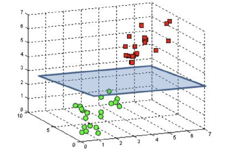
SVM is better than kNN model. It scales better. The model scales with number of features rather than the number of examples! Also, we explored the linear form of this model, i.e., the boundary separation is a linear function - a line in 2D or a plane in 3D or a hyperplane in n-D. We can use kernels to relax this and arrive at boundaries that are non-linear which allow us to express complex boundaries to discern between classes.

As part of visualizing the weights, I realized that maybe there is a better choice of regularization and learning rate constants. I came to this conclusion because my weights images do not make any sense. They make sense in a way that the images seem to be mirrored along y-axis indicating that the classifier is orientation invariant. If the image were more clear, I would be able to make a few more inferences regarding the general useful-ness of this model.

Right now, I get abot 34% as my accuracy on the testing dataset.

Future Directions

Some of the directions I would go about if given more times are –

• explore better ways to get learning rates and regularization constants. I had a buunch of values and iterated through every combination of them. Maybe a better way would be would to get values that along the gradient rather than only taking the values that I defined. This will make the training quite long compared to my implemented technique but since training will only happen a few times (compared to inference, this is worth it).

• Explore the use of non-linear models. There is a wealth of research on non-linear models based on guassian kernels and such and as an extension could look into these methods to improve the accuracy of the model.

Thanks!

Thanks for reading this article! For feedback and/or fanmail, send me an email 💌